CardioNIR — Predictive Modeling Pipeline
R/tidymodels Framework for Clinical Risk Prediction from NIRS, Biomarker, and Clinical Data
1 Overview
Work Package 6 (WP6) of the CardioNIR project developed a modular, reproducible R/tidymodels framework for clinical risk prediction integrating NIRS spectral data, molecular biomarkers (proteomic and metabolomic), and clinical variables. The pipeline covers the full analytical workflow from data ingestion through model evaluation, interpretability, and network analysis.
2 Pipeline Architecture
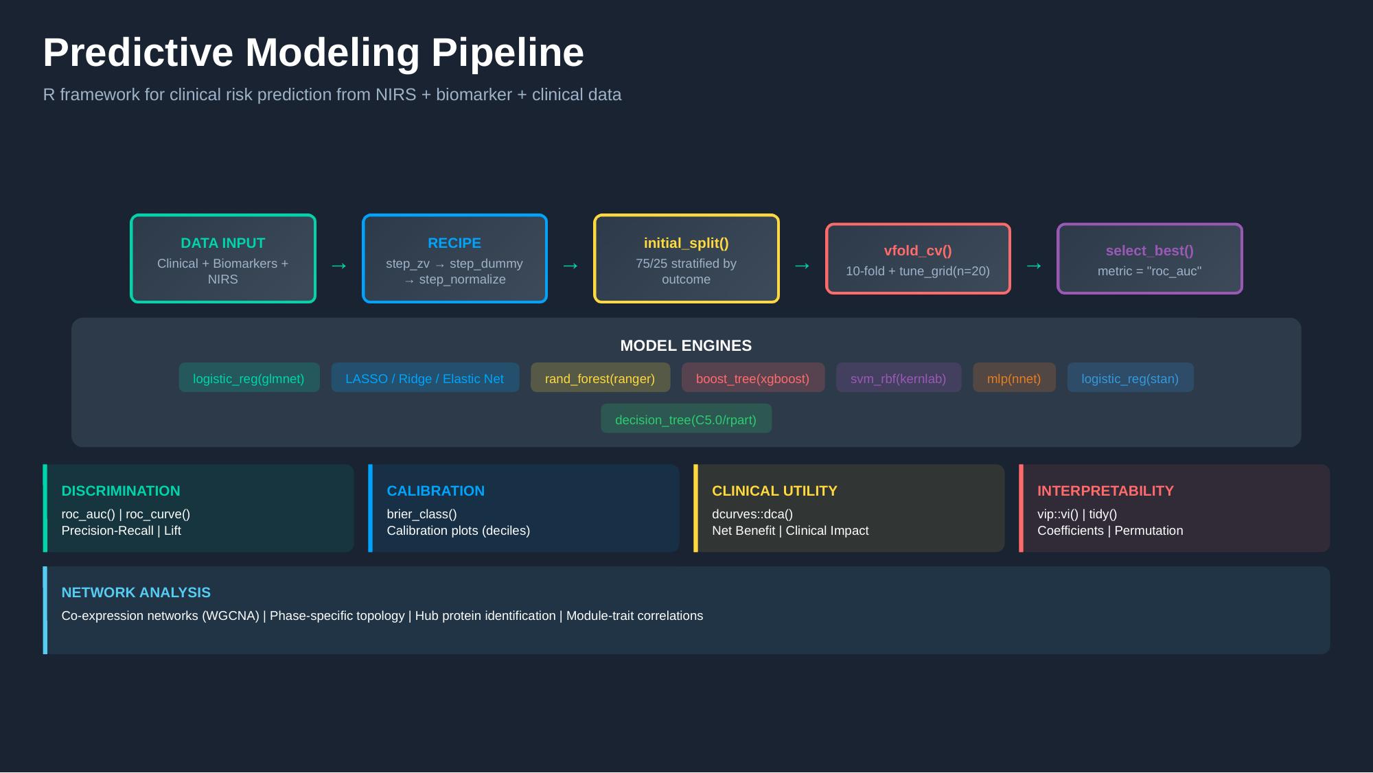
The pipeline is built entirely on the tidymodels ecosystem, ensuring a consistent grammar for model specification, preprocessing, tuning, and evaluation.
2.1 Stage 1: Data Input
The framework accepts three data modalities:
- Clinical variables — demographics, surgical parameters, comorbidities, haemodynamic measures
- Biomarkers — Olink proteomic NPX values (49 proteins), LC-MS metabolomic features (46 metabolites)
- NIRS spectra — SNV-transformed spectral features from the 900–1700 nm range
Data fusion strategies include early integration (feature concatenation), late integration (model stacking), and multi-block methods.
2.2 Stage 2: Preprocessing Recipe
Preprocessing is defined as a reproducible recipe() with the following steps:
recipe(outcome ~ ., data = training_data) |>
  step_zv(all_predictors()) |>        # Remove zero-variance features
  step_dummy(all_nominal()) |>         # Encode categorical variables
  step_normalize(all_numeric()) |>     # Centre and scale
  step_corr(threshold = 0.90) |>       # Optional: remove highly correlated
  step_pca(threshold = 0.95)           # Optional: dimensionality reduction
Additional steps for spectral data include step_ns() for basis expansion, step_filter_missing(), and custom spectral derivative steps.
2.3 Stage 3: Data Splitting
Stratified train/test splitting ensures balanced outcome representation:
initial_split(data, prop = 0.75, strata = outcome)2.4 Stage 4: Cross-Validation and Tuning
Hyperparameter tuning uses 10-fold cross-validation with a grid search of 20 candidate parameter sets:
vfold_cv(training_data, v = 10, strata = outcome)
tune_grid(resamples = folds, grid = 20, metrics = metric_set(roc_auc))
2.5 Stage 5: Model Selection
The best model is selected by select_best(metric = "roc_auc") and finalised with finalize_workflow() → last_fit().
3 Model Engines
The pipeline supports seven model families, all specified through the tidymodels interface:
| Engine | Function | Type | Key Hyperparameters |
|---|---|---|---|
| Elastic Net | logistic_reg(glmnet) |
Penalised regression | penalty, mixture (LASSO/Ridge/EN) |
| Random Forest | rand_forest(ranger) |
Ensemble | mtry, trees, min_n |
| XGBoost | boost_tree(xgboost) |
Gradient boosting | tree_depth, learn_rate, trees |
| SVM | svm_rbf(kernlab) |
Kernel methods | cost, rbf_sigma |
| Neural Net | mlp(nnet) |
Single-layer perceptron | hidden_units, penalty, epochs |
| Bayesian Logistic | logistic_reg(stan) |
Bayesian regression | Priors, chains, iter |
| Decision Tree | decision_tree(C5.0/rpart) |
Rule-based | cost_complexity, tree_depth |
All engines follow the same workflow() → tune_grid() → select_best() → last_fit() pattern, enabling systematic comparison across model families.
4 Evaluation Framework
Model evaluation is structured across four complementary dimensions:
4.1 Discrimination
Assessment of how well the model separates outcome classes:
roc_auc()androc_curve()— area under the ROC curve- Precision-Recall curves — particularly important for imbalanced outcomes
- Lift charts — clinical gain over random selection
4.2 Calibration
Assessment of whether predicted probabilities match observed frequencies:
brier_class()— Brier score for probability accuracy- Calibration plots (decile-based) — predicted vs. observed event rates
- Hosmer-Lemeshow goodness-of-fit
4.3 Clinical Utility
Translation of model predictions into clinical decision-making value:
dcurves::dca()— Decision Curve Analysis- Net Benefit across threshold probabilities
- Clinical Impact Curves — number of patients classified as high-risk vs. true positives at each threshold
4.4 Interpretability
Understanding which features drive predictions:
vip::vi()— variable importance (permutation-based and model-specific)tidy()— model coefficients for penalised regression- SHAP values (via
shapviz) — local and global feature contributions - Partial dependence plots
5 Network Analysis Module
Complementing the predictive modelling framework, the pipeline includes a dedicated network analysis module for co-expression analysis of proteomic and metabolomic data:
- WGCNA — Weighted Gene Co-expression Network Analysis adapted for protein/metabolite data
- Phase-specific topology — network construction at each surgical phase to capture dynamic rewiring
- Hub identification — degree centrality, betweenness, hub scores for identifying key molecular players
- Module-trait correlations — association of co-expression modules with clinical outcomes
This network module is the analytical engine behind the proteomics and metabolomics results pages.
6 Reusable Modules
The pipeline has been modularised into 22 reusable data analysis modules covering:
- Preprocessing and quality control
- Feature selection (stability selection, Boruta, recursive feature elimination)
- Model specification and tuning
- Evaluation and reporting
- Network construction and community detection
- Visualisation (volcano plots, heatmaps, PCA biplots, calibration plots)
These modules are currently deployed across active projects at the Cardiovascular Research Centre, including CardioNIR, BEACON, CARDIA, and IBERIA.